
A second-order system with a damping ratio of 0.3:
let s = poly([0, 1])
let G = 1 / (s * s + 0.6 * s + 1)

print(G)
print(poles(G))

let t = linspace(0, 20, 201)
plot(t, step(G, t))
Running it prints the transfer function, its poles and the step response:
       1
---------------
s^2 + 0.6 s + 1
(-0.3 + 0.953939i, -0.3 - 0.953939i)
1.5 ┤⠀⠀⠀⠀⠀⠀⠀⠀⠀⠀⠀⠀⠀⠀⠀⠀⠀⠀⠀⠀⠀⠀⠀⠀⠀⠀⠀⠀⠀⠀⠀⠀⠀⠀⠀⠀⠀⠀⠀⠀⠀⠀⠀⠀⠀⠀⠀⠀⠀⠀⠀⠀⠀⠀⠀⠀⠀⠀⠀⠀
    │⠀⠀⠀⠀⠀⠀⠀⠀⢠⠖⠲⢄⠀⠀⠀⠀⠀⠀⠀⠀⠀⠀⠀⠀⠀⠀⠀⠀⠀⠀⠀⠀⠀⠀⠀⠀⠀⠀⠀⠀⠀⠀⠀⠀⠀⠀⠀⠀⠀⠀⠀⠀⠀⠀⠀⠀⠀⠀⠀⠀
    │⠀⠀⠀⠀⠀⠀⠀⢰⠁⠀⠀⠀⠣⡀⠀⠀⠀⠀⠀⠀⠀⠀⠀⠀⠀⠀⠀⠀⠀⠀⠀⠀⠀⠀⠀⠀⠀⠀⠀⠀⠀⠀⠀⠀⠀⠀⠀⠀⠀⠀⠀⠀⠀⠀⠀⠀⠀⠀⠀⠀
    │⠀⠀⠀⠀⠀⠀⢀⠇⠀⠀⠀⠀⠀⠱⡀⠀⠀⠀⠀⠀⠀⠀⠀⠀⠀⠀⠀⠀⠀⠀⠀⠀⠀⠀⠀⠀⠀⠀⠀⠀⠀⠀⠀⠀⠀⠀⠀⠀⠀⠀⠀⠀⠀⠀⠀⠀⠀⠀⠀⠀
    │⠀⠀⠀⠀⠀⠀⡎⠀⠀⠀⠀⠀⠀⠀⠈⢆⠀⠀⠀⠀⠀⠀⠀⠀⠀⠀⣀⡤⠤⠤⠤⠤⢤⣀⣀⡀⠀⠀⠀⠀⠀⠀⠀⠀⠀⠀⢀⣀⣀⣀⣀⣀⡀⠀⠀⠀⠀⠀⠀⠀
1.0 ┤⠀⠀⠀⠀⠀⢰⠁⠀⠀⠀⠀⠀⠀⠀⠀⠀⠳⣀⠀⠀⠀⠀⢀⡤⠞⠉⠀⠀⠀⠀⠀⠀⠀⠀⠀⠉⠉⠉⠉⠉⠉⠉⠉⠉⠉⠉⠉⠀⠀⠀⠀⠀⠈⠉⠉⠉⠉⠉⠉⠉
    │⠀⠀⠀⠀⠀⡎⠀⠀⠀⠀⠀⠀⠀⠀⠀⠀⠀⠈⠑⠒⠒⠋⠁⠀⠀⠀⠀⠀⠀⠀⠀⠀⠀⠀⠀⠀⠀⠀⠀⠀⠀⠀⠀⠀⠀⠀⠀⠀⠀⠀⠀⠀⠀⠀⠀⠀⠀⠀⠀⠀
    │⠀⠀⠀⠀⢠⠃⠀⠀⠀⠀⠀⠀⠀⠀⠀⠀⠀⠀⠀⠀⠀⠀⠀⠀⠀⠀⠀⠀⠀⠀⠀⠀⠀⠀⠀⠀⠀⠀⠀⠀⠀⠀⠀⠀⠀⠀⠀⠀⠀⠀⠀⠀⠀⠀⠀⠀⠀⠀⠀⠀
    │⠀⠀⠀⠀⡎⠀⠀⠀⠀⠀⠀⠀⠀⠀⠀⠀⠀⠀⠀⠀⠀⠀⠀⠀⠀⠀⠀⠀⠀⠀⠀⠀⠀⠀⠀⠀⠀⠀⠀⠀⠀⠀⠀⠀⠀⠀⠀⠀⠀⠀⠀⠀⠀⠀⠀⠀⠀⠀⠀⠀
0.5 ┤⠀⠀⠀⢠⠃⠀⠀⠀⠀⠀⠀⠀⠀⠀⠀⠀⠀⠀⠀⠀⠀⠀⠀⠀⠀⠀⠀⠀⠀⠀⠀⠀⠀⠀⠀⠀⠀⠀⠀⠀⠀⠀⠀⠀⠀⠀⠀⠀⠀⠀⠀⠀⠀⠀⠀⠀⠀⠀⠀⠀
    │⠀⠀⠀⡸⠀⠀⠀⠀⠀⠀⠀⠀⠀⠀⠀⠀⠀⠀⠀⠀⠀⠀⠀⠀⠀⠀⠀⠀⠀⠀⠀⠀⠀⠀⠀⠀⠀⠀⠀⠀⠀⠀⠀⠀⠀⠀⠀⠀⠀⠀⠀⠀⠀⠀⠀⠀⠀⠀⠀⠀
    │⠀⠀⢠⠃⠀⠀⠀⠀⠀⠀⠀⠀⠀⠀⠀⠀⠀⠀⠀⠀⠀⠀⠀⠀⠀⠀⠀⠀⠀⠀⠀⠀⠀⠀⠀⠀⠀⠀⠀⠀⠀⠀⠀⠀⠀⠀⠀⠀⠀⠀⠀⠀⠀⠀⠀⠀⠀⠀⠀⠀
    │⠀⠀⡸⠀⠀⠀⠀⠀⠀⠀⠀⠀⠀⠀⠀⠀⠀⠀⠀⠀⠀⠀⠀⠀⠀⠀⠀⠀⠀⠀⠀⠀⠀⠀⠀⠀⠀⠀⠀⠀⠀⠀⠀⠀⠀⠀⠀⠀⠀⠀⠀⠀⠀⠀⠀⠀⠀⠀⠀⠀
    │⠀⢀⠇⠀⠀⠀⠀⠀⠀⠀⠀⠀⠀⠀⠀⠀⠀⠀⠀⠀⠀⠀⠀⠀⠀⠀⠀⠀⠀⠀⠀⠀⠀⠀⠀⠀⠀⠀⠀⠀⠀⠀⠀⠀⠀⠀⠀⠀⠀⠀⠀⠀⠀⠀⠀⠀⠀⠀⠀⠀
0.0 ┤⣠⠃⠀⠀⠀⠀⠀⠀⠀⠀⠀⠀⠀⠀⠀⠀⠀⠀⠀⠀⠀⠀⠀⠀⠀⠀⠀⠀⠀⠀⠀⠀⠀⠀⠀⠀⠀⠀⠀⠀⠀⠀⠀⠀⠀⠀⠀⠀⠀⠀⠀⠀⠀⠀⠀⠀⠀⠀⠀⠀
    └┬──────────────┬──────────────┬─────────────┬──────────────┬
     0              5             10            15             20
The same plot can be saved as an SVG file with plot_svg,
or opened in your browser with show:
plot_svg(t, step(G, t), "step.svg")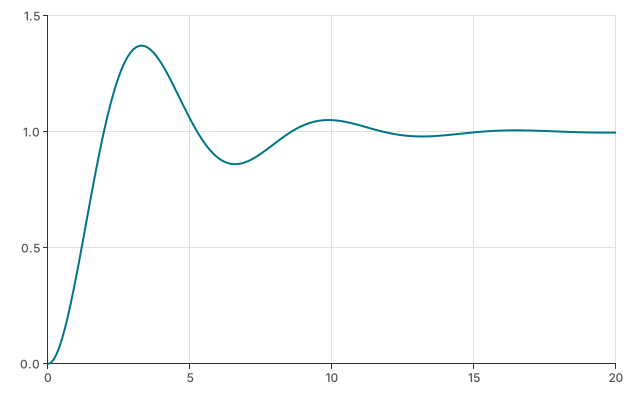
In the REPL
Polynomials and transfer functions are ordinary values, and they print as fractions.
aktua> let p = poly([1, 2, 3])
aktua> 1/p

       1
---------------
3 s^2 + 2 s + 1

aktua> poles(1/p)

(-0.333333 + 0.471405i, -0.333333 - 0.471405i)
Vectors and matrices
Commas separate elements and semicolons separate rows.
Arithmetic works element by element, @ is the matrix
product and .T transposes.
aktua> let a = [1, 2, 3]
aktua> let M = [1, 2, 3; 4, 5, 6]
aktua> M @ a

[14, 32]

aktua> a.T * a

[[1, 2, 3],
 [2, 4, 6],
 [3, 6, 9]]
Transfer functions can be evaluated on whole vectors, so a frequency response is one line:
aktua> let s = poly([0, 1])
aktua> let G = 1 / (s + 1)
aktua> let j = complex(0, 1)
aktua> abs(G(j * [0.1, 1, 10]))

[ 0.995037,  0.707107, 0.0995037]
Simulating your own dynamics
Not everything is a transfer function. A tank whose outflow follows
Torricelli's law, A dh/dt = q_in - k sqrt(h), is nonlinear,
but a Runge-Kutta step is a few lines of Aktua:
let A    = 2       // Cross-section [m^2]
let k    = 0.02    // Outflow coefficient [m^2.5/s]
let q_in = 0.01    // Inflow [m^3/s]

fn f(t, h) { (q_in - k * sqrt(h)) / A }

// One step of classic Runge-Kutta
fn rk4(f, t, y, dt) {
  let k1 = f(t, y)
  let k2 = f(t + dt/2, y + dt/2 * k1)
  let k3 = f(t + dt/2, y + dt/2 * k2)
  let k4 = f(t + dt, y + dt * k3)
  y + dt/6 * (k1 + 2*k2 + 2*k3 + k4)
}

let t = linspace(0, 500, 501)
let h = zeros([len(t)])
for i in range(1, len(t)) {
  h[i] = rk4(f, t[i-1], h[i-1], t[i] - t[i-1])
}

print("Final level: " + h[-1] + " m, steady state " + (q_in / k)^2 + " m")
plot(t, h)
Final level: 0.248759 m, steady state 0.25 m
0.3 ┤⠀⠀⠀⠀⠀⠀⠀⠀⠀⠀⠀⠀⠀⠀⠀⠀⠀⠀⠀⠀⠀⠀⠀⠀⠀⠀⠀⠀⠀⠀⠀⠀⠀⠀⠀⠀⠀⠀⠀⠀⠀⠀⠀⠀⠀⠀⠀⠀⠀⠀⠀⠀⠀⠀⠀⠀⠀⠀⠀⠀
│⠀⠀⠀⠀⠀⠀⠀⠀⠀⠀⠀⠀⠀⠀⠀⠀⠀⠀⠀⠀⠀⠀⠀⠀⠀⠀⠀⠀⠀⠀⠀⠀⠀⠀⠀⠀⠀⠀⠀⠀⠀⠀⠀⠀⠀⠀⠀⠀⠀⠀⠀⠀⠀⠀⠀⠀⠀⠀⠀⠀
│⠀⠀⠀⠀⠀⠀⠀⠀⠀⠀⠀⠀⠀⠀⠀⠀⠀⠀⠀⠀⠀⠀⠀⠀⠀⠀⠀⠀⠀⠀⠀⠀⠀⠀⠀⠀⠀⣀⣀⣀⣀⣀⣀⣀⣀⣀⣀⣠⠤⠤⠤⠤⠤⠤⠤⠤⠤⠤⠤⠤
│⠀⠀⠀⠀⠀⠀⠀⠀⠀⠀⠀⠀⠀⠀⠀⠀⠀⠀⠀⠀⠀⠀⢀⣀⣀⠤⠤⠴⠒⠒⠒⠊⠉⠉⠉⠉⠉⠀⠀⠀⠀⠀⠀⠀⠀⠀⠀⠀⠀⠀⠀⠀⠀⠀⠀⠀⠀⠀⠀⠀
│⠀⠀⠀⠀⠀⠀⠀⠀⠀⠀⠀⠀⠀⠀⠀⠀⢀⣠⠤⠖⠚⠉⠉⠀⠀⠀⠀⠀⠀⠀⠀⠀⠀⠀⠀⠀⠀⠀⠀⠀⠀⠀⠀⠀⠀⠀⠀⠀⠀⠀⠀⠀⠀⠀⠀⠀⠀⠀⠀⠀
0.2 ┤⠀⠀⠀⠀⠀⠀⠀⠀⠀⠀⠀⠀⢀⡠⠔⠋⠉⠀⠀⠀⠀⠀⠀⠀⠀⠀⠀⠀⠀⠀⠀⠀⠀⠀⠀⠀⠀⠀⠀⠀⠀⠀⠀⠀⠀⠀⠀⠀⠀⠀⠀⠀⠀⠀⠀⠀⠀⠀⠀⠀
│⠀⠀⠀⠀⠀⠀⠀⠀⠀⠀⡠⠖⠉⠀⠀⠀⠀⠀⠀⠀⠀⠀⠀⠀⠀⠀⠀⠀⠀⠀⠀⠀⠀⠀⠀⠀⠀⠀⠀⠀⠀⠀⠀⠀⠀⠀⠀⠀⠀⠀⠀⠀⠀⠀⠀⠀⠀⠀⠀⠀
│⠀⠀⠀⠀⠀⠀⠀⢀⡴⠋⠀⠀⠀⠀⠀⠀⠀⠀⠀⠀⠀⠀⠀⠀⠀⠀⠀⠀⠀⠀⠀⠀⠀⠀⠀⠀⠀⠀⠀⠀⠀⠀⠀⠀⠀⠀⠀⠀⠀⠀⠀⠀⠀⠀⠀⠀⠀⠀⠀⠀
│⠀⠀⠀⠀⠀⠀⡴⠋⠀⠀⠀⠀⠀⠀⠀⠀⠀⠀⠀⠀⠀⠀⠀⠀⠀⠀⠀⠀⠀⠀⠀⠀⠀⠀⠀⠀⠀⠀⠀⠀⠀⠀⠀⠀⠀⠀⠀⠀⠀⠀⠀⠀⠀⠀⠀⠀⠀⠀⠀⠀
0.1 ┤⠀⠀⠀⠀⢀⠞⠀⠀⠀⠀⠀⠀⠀⠀⠀⠀⠀⠀⠀⠀⠀⠀⠀⠀⠀⠀⠀⠀⠀⠀⠀⠀⠀⠀⠀⠀⠀⠀⠀⠀⠀⠀⠀⠀⠀⠀⠀⠀⠀⠀⠀⠀⠀⠀⠀⠀⠀⠀⠀⠀
│⠀⠀⠀⣠⠋⠀⠀⠀⠀⠀⠀⠀⠀⠀⠀⠀⠀⠀⠀⠀⠀⠀⠀⠀⠀⠀⠀⠀⠀⠀⠀⠀⠀⠀⠀⠀⠀⠀⠀⠀⠀⠀⠀⠀⠀⠀⠀⠀⠀⠀⠀⠀⠀⠀⠀⠀⠀⠀⠀⠀
│⠀⠀⣰⠃⠀⠀⠀⠀⠀⠀⠀⠀⠀⠀⠀⠀⠀⠀⠀⠀⠀⠀⠀⠀⠀⠀⠀⠀⠀⠀⠀⠀⠀⠀⠀⠀⠀⠀⠀⠀⠀⠀⠀⠀⠀⠀⠀⠀⠀⠀⠀⠀⠀⠀⠀⠀⠀⠀⠀⠀
│⠀⢰⠃⠀⠀⠀⠀⠀⠀⠀⠀⠀⠀⠀⠀⠀⠀⠀⠀⠀⠀⠀⠀⠀⠀⠀⠀⠀⠀⠀⠀⠀⠀⠀⠀⠀⠀⠀⠀⠀⠀⠀⠀⠀⠀⠀⠀⠀⠀⠀⠀⠀⠀⠀⠀⠀⠀⠀⠀⠀
│⢠⠇⠀⠀⠀⠀⠀⠀⠀⠀⠀⠀⠀⠀⠀⠀⠀⠀⠀⠀⠀⠀⠀⠀⠀⠀⠀⠀⠀⠀⠀⠀⠀⠀⠀⠀⠀⠀⠀⠀⠀⠀⠀⠀⠀⠀⠀⠀⠀⠀⠀⠀⠀⠀⠀⠀⠀⠀⠀⠀
0.0 ┤⡎⠀⠀⠀⠀⠀⠀⠀⠀⠀⠀⠀⠀⠀⠀⠀⠀⠀⠀⠀⠀⠀⠀⠀⠀⠀⠀⠀⠀⠀⠀⠀⠀⠀⠀⠀⠀⠀⠀⠀⠀⠀⠀⠀⠀⠀⠀⠀⠀⠀⠀⠀⠀⠀⠀⠀⠀⠀⠀⠀
└┬───────────┬───────────┬──────────┬───────────┬───────────┬
0 100 200 300 400 500
What it has so far
- Polynomials and transfer functions, with arithmetic between them
- Poles, and impulse and step responses of LTI systems
- Discrete-time transfer functions, in
z - Real and complex numbers, with the usual math functions
- Vectors and matrices, with broadcasting, transposes and a matrix product
- Functions, loops, conditionals and imports, enough to write your own ODE solvers
- Line plots, drawn in the terminal with braille characters or saved as SVG files
- An interactive REPL, or scripts run from the command line
Aktua is experimental. Expect missing features, rough error messages and breaking changes.
Building it
You need a C compiler and make.
git clone https://github.com/marciorvneto/aktua
cd aktua
make
./build/aktua examples/leaky_tank.akt
Run ./build/aktua with no arguments to start the REPL.